Machine learning algorithms and the art of hyperparameter selection

Machine learning algorithms are used everywhere from a smartphone to a spacecraft. They tell you the weather forecast for tomorrow, translate from one language into another, and suggest what TV series you might like next on Netflix.

These algorithms automatically adjust (learn) their internal parameters based on data. However, there is a subset of parameters that is not learned and that have to be configured by an expert. Such parameters are often referred to as “hyperparameters” — and they have a big impact on our lives as the use of AI increases.

For example, the tree depth in a decision tree model and the number of layers in an artificial neural network are typical hyperparameters. The performance of a model can drastically depend on the choice of its hyperparameters. A decision tree can yield good results for moderate tree depth and have very bad performance for very deep trees.

The choice of the optimal hyperparameters is more art than science, if we want to run it manually. Indeed, the optimal selection of the hyperparameter values depends on the problem at hand.

Since the algorithms, the goals, the data types, and the data volumes change considerably from one project to another, there is no single best choice for hyperparameter values that fits all models and all problems. Instead, hyperparameters must be optimized within the context of each machine learning project.

In this article, we’ll start with a review of the power of an optimization strategy and then provide an overview of four commonly used optimization strategies:

• Grid search
• Random search
• Hill climbing
• Bayesian optimization

The optimization strategy

Even with in-depth domain knowledge by an expert, the task of manual optimization of the model hyperparameters can be very time-consuming. An alternative approach is to set aside the expert and adopt an automatic approach. An automatic procedure to detect the optimal set of hyperparameters for a given model in a given project in terms of some performance metric is called an optimization strategy.

A typical optimization procedure defines the possible set of hyperparameters and the metric to be maximized or minimized for that particular problem. Hence, in practice, any optimization procedure follows these classical steps:

• 1) Split the data at hand into training and test subsets
• 2) Repeat optimization loop a fixed number of times or until a condition is met:
  • a) Select a new set of model hyperparameters
  • b) Train the model on the training subset using the selected set of hyperparameters
  • c) Apply the model to the test subset and generate the corresponding predictions
  • d) Evaluate the test predictions using the appropriate scoring metric for the problem at hand, such as accuracy or mean absolute error. Store the metric value that corresponds to the selected set of hyperparameters
• 3) Compare all metric values and choose the hyperparameter set that yields the best metric value

The question is how to pass from step 2d back to step 2a for the next iteration; that is, how to select the next set of hyperparameters, making sure that it is actually better than the previous set. We would like our optimization loop to move toward a reasonably good solution, even though it may not be the optimal one. In other words, we want to be reasonably sure that the next set of hyperparameters is an improvement over the previous one.

A typical optimization procedure treats a machine learning model as a black box. That means at each iteration for each selected set of hyperparameters, all we are interested in is the model performance as measured by the selected metric. We do not need (want) to know what kind of magic happens inside the black box. We just need to move to the next iteration and iterate over the next performance evaluation, and so on.

The key factor in all different optimization strategies is how to select the next set of hyperparameter values in step 2a, depending on the previous metric outputs in step 2d. Therefore, for a simplified experiment, we omit the training and testing of the black box, and we focus on the metric calculation (a mathematical function) and the strategy to select the next set of hyperparameters. In addition, we have substituted the metric calculation with an arbitrary mathematical function and the set of model hyperparameters with the function parameters.

In this way, the optimization loop runs faster and remains as general as possible. One further simplification is to use a function with only one hyperparameter to allow for an easy visualization. Below is the function we used to demonstrate the four optimization strategies. We would like to emphasize that any other mathematical function would have worked as well.

f(x) = sin(x/2) + 0.5⋅sin(2⋅x) +0.25⋅cos(4.5⋅x)

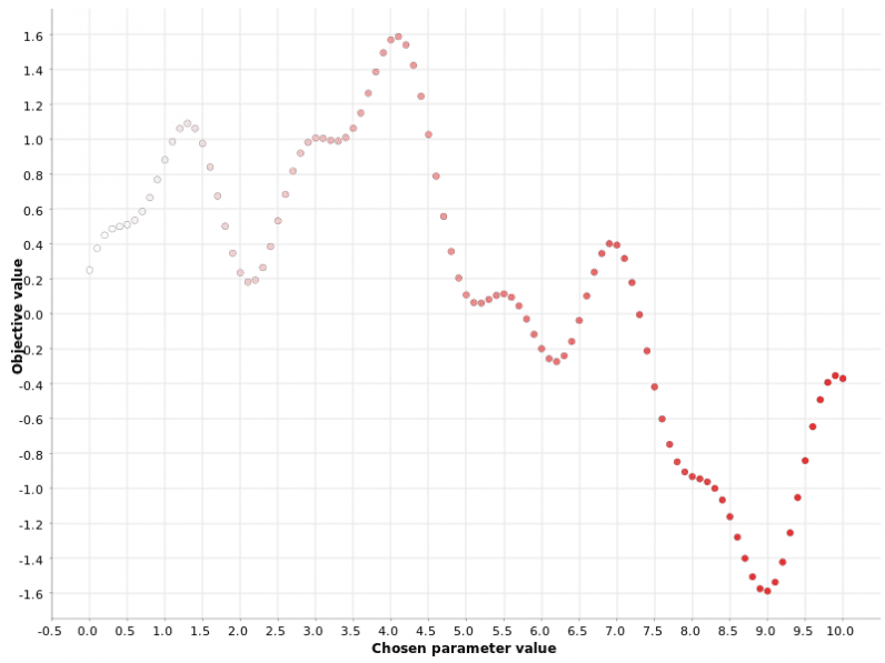
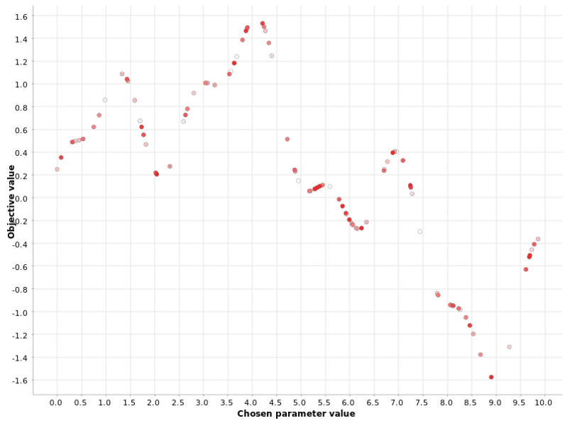
This simplified setup allows us to visualize the experimental values of the one hyperparameter and the corresponding function values on a simple x-y plot. On the x axis are the hyperparameter values and on the y axis the function outputs. The (x,y) points are then colored according to a white-red gradient describing the point position in the generation of the hyperparameter sequence.

Whiter points correspond to hyperparameter values generated earlier in the process; redder points correspond to hyperparameter values generated later on in the process. This gradient coloring will be useful later to illustrate the differences across the optimization strategies.

The goal of the optimization procedure in this simplified use case is to find the one hyperparameter that maximizes the value of the function.

Let’s begin our review of four common optimization strategies used to identify the new set of hyperparameter values for the next iteration of the optimization loop.

Grid search

This is a basic brute-force strategy. If you do not know which values to try, you try them all. All possible values within a range with a fixed step are used in the function evaluation.

For example, if the range is [0, 10] and the step size is 0.1, then we would get the sequence of hyperparameter values (0, 0.1, 0.2, 0.3, … 9.5, 9.6, 9.7, 9.8, 9.9, 10). In a grid search strategy, we calculate the function output for each and every one of these hyperparameter values. Therefore, the finer the grid, the closer we get to the optimum — but also the higher the required computation resources.

The grid search strategy can work well in the case of a single parameter, but it becomes very inefficient when multiple parameters have to be optimized simultaneously.

Random search

For the random search strategy, the values of the hyperparameters are selected randomly, as the name suggests. This strategy is typically preferred in the case of multiple hyperparameters, and it is particularly efficient when some hyperparameters affect the final metric more than others.

Again, the hyperparameter values are generated within a range [0, 10]. Then, a fixed number N of hyperparameters is randomly generated. The fixed number N of predefined hyperparameters to experiment with allows you to control the duration and speed of this optimization strategy. The larger the N, the higher the probability to get to the optimum — but also the higher the required computation resources.

Hill climbing

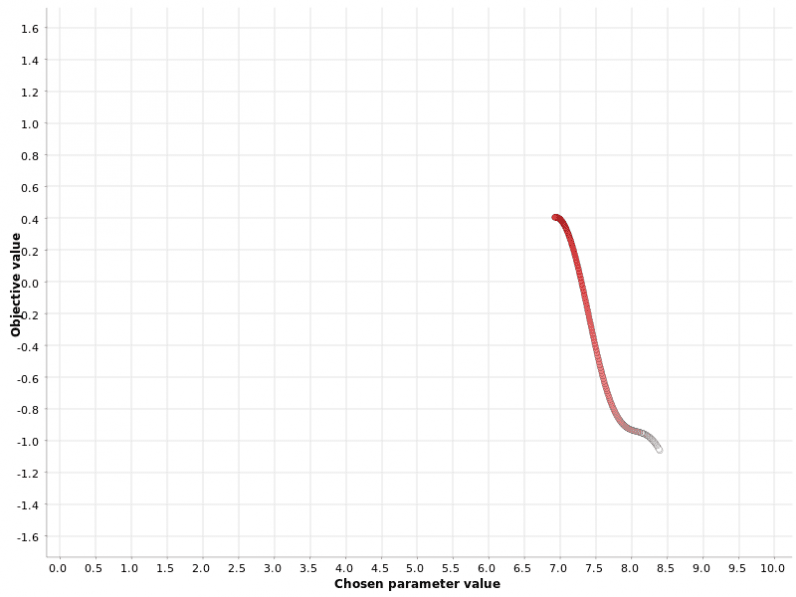
The hill climbing approach at each iteration selects the best direction in the hyperparameter space to choose the next hyperparameter value. If no neighbor improves the final metric, the optimization loop stops.

Note that this procedure is different from the grid and random searches in one important aspect: selection of the next hyperparameter value takes into account the outcomes of previous iterations.

This example illustrates a caveat related to this strategy: it can get stuck in a secondary maximum. From the other plots, we can see that the global maximum is located at x=4.0 with corresponding metric value of 1.6. This strategy does not find the global maximum but gets stuck into a local one. A good rule of thumb for this method is to run it multiple times with different starting values and to check whether the algorithm converges to the same maximum.

Bayesian optimization

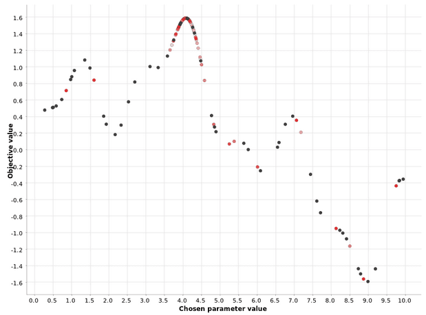
The Bayesian optimization strategy selects the next hyperparameter value based on the function outputs in the previous iterations, similar to the hill climbing strategy. Unlike hill climbing, Bayesian optimization looks at past iterations globally and not only at the last one.

There are typically two phases in this procedure:

• During the first phase, called warm-up, hyperparameter values are generated randomly. After a user-defined number N of such random generations of hyperparameters, the second phase kicks in.
• In the second phase, at each iteration, a “surrogate” model of type P(output | past hyperparameters) is estimated to describe the conditional probability of the output values on the hyperparameter values from past iterations. This surrogate model is much easier to optimize than the original function. Thus, the algorithm optimizes the surrogate and suggests the hyperparameter values at the maximum of the surrogate model as the optimal values for the original function as well. A fraction of the iterations in the second phase is also used to probe areas outside of the optimal region. This is to avoid the problem of local maxima.

You can also see that intense red points are clustered closer to the maximum, while pale red and white points are scattered. This demonstrates that the definition of the optimal region is improved with each iteration of the second phase.

Summary

We all know the importance of hyperparameter optimization while training a machine learning model. Since manual optimization is time-consuming and requires specific expert knowledge, we have explored four common automatic procedures for hyperparameter optimization.

In general, an automatic optimization procedure follows an iterative procedure in which at each iteration, the model is trained on a new set of hyperparameters and evaluated on the test set. At the end, the hyperparameter set corresponding to the best metric score is chosen as the optimal set. The question is how to select the next set of hyperparameters, ensuring that this is actually better than the previous set.

We have provided an overview of four commonly used optimization strategies: grid search, random search, hill climbing, and Bayesian optimization. They all have pros and cons, and we have briefly explained the differences by illustrating how they work on a simple toy use case. Now you are all set to go and try them out in a real-world machine learning problem.